Apr 26, 2018
Speeding up your code: creating NumPy universal functions with Numba
If you want to play with the code, the notebook is available here
I have read recently this very interesting series of articles about how one can speed up code written in Python.
I encourage you to go read the full series if you want more details, especially on how to use parallelisation and just-in-time compiling to speed up your code.
I want to focus here on the first trick presented, that of vectorizing your code with NumPy, instead of using Python loops and iterators. Don’t get me wrong, I love Python iterators and their expressive power, but for numerical computations, they just won’t do the job.
Vectorizing your computation can give you a speedup of several orders of magnitude. However, this vectorizing step can sometimes be non-trivial, and requires quite a lot of work, of NumPy twisting and handling harrowing concepts such as strides. This in turn makes your code less understandable and less easily maintainable. But what wouldn’t we do for a factor-100 speedup?
What I want to test here is how large a speedup can we gain without vectorizing our Python code, but instead by using Numba to define a (compiled) universal function for NumPy.
Universal functions are vectorized functions operating elementwise on NumPy arrays. One can think of functions such as np.exp or np.power. NumPy contains quite a lot of the most usually needed functions, but Numba allows you to define your own through the decorator @vectorize.
It is far more efficient than using np.apply, which performs a for-loop underneath. On the other hand, vectorized functions defined with Numba are compiled, and should be more efficient. Let’s find out how fast we can get without vectorizing by hand.
Generate data
First, I generated some data to reproduce the results exposed in the aforementioned article.
import numpy as np

N = 1000
r = np.random.uniform(0, 1, size=N)
theta = np.random.uniform(0, 2*np.pi, size=N)
data  = np.vstack((r * np.cos(theta), r * np.sin(theta))).T
We can plot the sample data.
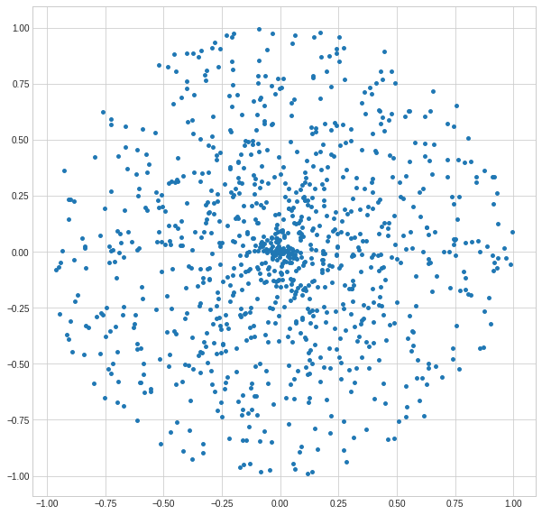
Looks good. Now, let’s try to clusterize it in a Poincaré ball space (using a non-Euclidean distance).
Naive Python implementation
First, as a baseline, I run the naive (almost) pure Python implementation.
The _dist_poinc function computes the needed distance between two points (represented as NumPy arrays).
Then, for each point, we compute the distance to every other point through a loop in dist_poinc. We apply the meanshift algorithm for each point (see the original article for more details): each point is shifted toward the mean of similar (i.e. close enough) points. How close is close enough is parametrized by the sigma value.
def _dist_poinc(a, b):
    num=np.dot(a-b, a-b)
    den1=1-np.dot(a,a)
    den2=1-np.dot(b,b)
    return np.arccosh(1+ 2* (num) / (den1*den2))

def dist_poinc(a, B):
    return np.array([_dist_poinc(a, b) for b in B])

def gaussian(d, bw):
    return np.exp(-0.5*(d/bw)**2) / (bw*np.sqrt(2*np.pi))

def meanshift(points, sigma):
    shifted_pts = np.empty(points.shape)
    for i, p in enumerate(points):
        dists = dist_poinc( p, points)
        weights = gaussian(dists, sigma)
        shifted_pts[i] = (np.expand_dims(weights,1) * points).sum(0) / weights.sum()
    return shifted_pts
%timeit meanshift(data, .2)
5.51 s ± 268 ms per loop (mean ± std. dev. of 7 runs, 1 loop each)
Each iteration of this algorithm takes roughly 6 seconds on 1000 points, which is slow.
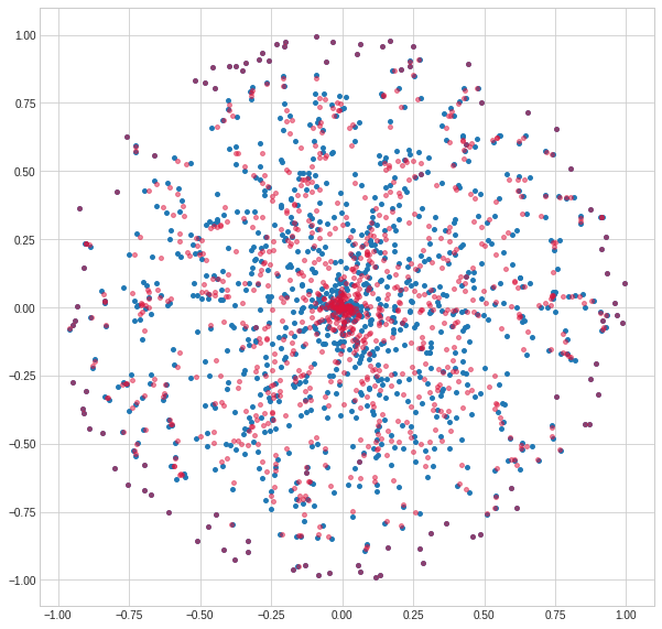
We can plot the shifted points, and see how they start to cluster in the centre (and not at all on the periphery, because of the use of the Poincaré distance).
clustered = meanshift(data, .2)
Vectorized NumPy implementation
Next, we can see how the vectorized implementation is performing. For detail on how it is derived, I refer you to the original article, as it is not in the scope of this experiment.
def num(points):
    expd = np.expand_dims(points,2)
    tiled = np.tile(expd, points.shape[0])
    return np.sum(np.square(points.T - tiled ), axis=1)

def den(points):
    sq_norm = 1 - np.sum(np.square(points), 1)
    expd = np.expand_dims(sq_norm, 1)
    return expd * expd.T

def poinc_dist_vec(points):
    return np.arccosh(1 + 2 * num(points)/ den(points))

def gaussian(d, bw):
    return np.exp(-0.5*(d/bw)**2) / (bw*np.sqrt(2*np.pi))

def meanshift_vec(points, sigma):
    dists = poinc_dist_vec(points)
    weights = gaussian(dists, sigma)
    expd_w = np.dot(weights, points)
    summed_weights = np.sum(weights, 0)
    shifted_pts = expd_w / np.expand_dims(summed_weights, 1)
    return shifted_pts
We can check that we get the same results as in the original implementation, up to a small numerical precision error.
clustered_vec = meanshift_vec(data, .2)
np.allclose(clustered_vec, clustered)  # True
%timeit meanshift_vec(data, .2)
85.9 ms ± 873 µs per loop (mean ± std. dev. of 7 runs, 10 loops each)
With this implementation, each iteration is taking roughly 85 ms, a speedup by a factor 70. It is definitely worth the slightly less readable code.
Numba JIT implementation
What I want to know is how fast can my implementation be using the definition of the distance in Python, and just-in-time compiling with Numba.
We write down the same function as in the first implementation (we just expand the np.dot to work with scalars instead of vectors), and we use the @vectorize decorator to create a ufunc.
Then, we can compute all distances in one line, after computing the Cartesian product of all possible pairs of point, and reshape it in the distance matrix.
The rest of the implementation is the same as the vectorized NumPy implementation.
from numba import vectorize, float64

@vectorize([float64(float64, float64, float64, float64)])
def dist_poinc_jit(a1, a2, b1, b2):
    num = np.power(a1 - b1, 2) + np.power(a2 - b2, 2)
    den1 = 1 - (np.power(a1, 2) + np.power(a2, 2))
    den2 = 1 - (np.power(b1, 2) + np.power(b2, 2))
    return np.arccosh(1+ 2* (num) / (den1*den2))

def cartesian_product(arr1, arr2):
    return np.hstack((np.repeat(arr1, len(arr2), axis=0), np.concatenate(len(arr1) * [arr2])))

def gaussian(d, bw):
    return np.exp(-0.5*(d/bw)**2) / (bw*np.sqrt(2*np.pi))

def meanshift_numba(points, sigma):
    dists = dist_poinc_jit(*cartesian_product(points, points).T).reshape((len(points), len(points)))
    weights = gaussian(dists, sigma)
    expd_w = np.dot(weights, points)
    summed_weights = np.sum(weights, 0)
    shifted_pts = expd_w / np.expand_dims(summed_weights, 1)
    return shifted_pts
Once again, we can check that we get the same result as before.
clustered_jit = meanshift_numba(data, .2)
np.allclose(clustered_vec, clustered_jit)  # True
%timeit meanshift_numba(data, .2)
102 ms ± 271 µs per loop (mean ± std. dev. of 7 runs, 10 loops each)
This implementation is taking roughly 100 ms per iteration, which is a bit slower than the vectorized implementation in NumPy, but much faster than the first implementation with Python loops.
If your code is too complex to be vectorized, or if you do not care so much for raw performance as for readability, just-in-time compiling with Numba is a great option you should consider.